Statistical Learning 

Introduction:

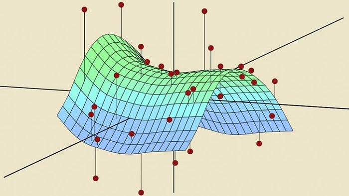
While I’ve talked a lot about the different types of machine learning algorithms, I’d like to spend some time giving an overview of Statistical Learning theory for those who may be confused. Statistical learning theory is a framework for machine learning that draws from statistics and functional analysis. It deals with finding a predictive function based on the data presented. The main idea in statistical learning theory is to build a model that can draw conclusions from data and make predictions.

Types of Data in Statistical Learning:

With statistical learning theory, there are two main types of data:

• Dependent Variable — a variable (y) whose values depend on the values of other variables (a dependent variable is sometimes also referred to as a target variable)
• Independent Variables — a variable (x) whose value does not depend on the values of other variables (independent variables are sometimes also referred to as predictor variables, input variables, explanatory variables, or features)

In statistical learning, the independent variable(s) are the variable that will affect the dependent variable.

A common examples of an Independent Variable is Age. There is nothing that one can do to increase or decrease age. This variable is independent.

Some common examples of Dependent Variables are:

• Weight — a person’s weight is dependent on his or her age, diet, and activity levels (as well as other factors)
• Temperature — temperature is impacted by altitude, distance from equator (latitude) and distance from the sea

In graphs, the independent variable is often plotted along the x-axis while the dependent variable is plotted along the y-axis.

In this example, which shows how the price of a home is affected by the size of the home, sq. ft is the independent variable while price of the home is the dependent variable.

Statistical Model:

A statistical model defines the relationships between a dependent and independent variable. In the above graph, the relationships between the size of the home and the price of the home is illustrated by the straight line. We can define this relationship by using y = mx + c where m represents the gradient and c is the intercept. Another way that this equation can be expressed is with roman numerals which would look something like:

This model would describe the price of a home as having a linear relationship with the size of a home. This would represent a simple model for the relationship.

If we suppose that the size of the home is not the only independent variable when determining the price and that the number of bathrooms is also an independent variable, the equation would look like:

Model Generalization:

In order to build an effective model, the available data needs to be used in a way that would make the model generalizable for unseen situations. Some problems that occur when building models is that the model under-fits or over-fits to the data.

• Under-fitting — when a statistical model does not adequately capture the underlying structure of the data and, therefore, does not include some parameters that would appear in a correctly specified model.
• Over-fitting — when a statistical model contains more parameters that can be justified by the data and includes the residual variation (“noise”) as if the variation represents underlying model structure.

As you can see, it is important to create a model that can generalize to the data that it is given so that it can make the most accurate predictions when given new data.

Model Validation:

Model Validation is used to assess over-fitting and under-fitting of the data. The steps to perform model validation are:

1. Split the data into two parts, training data and testing data (anywhere between 80/20 and 70/30 is ideal)
2. Use the larger portion (training data) to train the model
3. Use the smaller portion (testing data) to test the model. This data is not being used to train the model, so it will be new data for the model to build predictions from.
4. If the model has learned well from the training data, it will perform well with both the training data and testing data. To determine how well the model is performing on both sets of data, you can calculate the accuracy score for each. The model is over-fitting if the training data has a significantly higher accuracy score than the testing data.